The binomial model is a simple yet effective pricing model. In this article we will explain the math behind the binomial pricing model, develop a Python script to implement it and finally test it out on some real market data from Yahoo Finance.
We will also show the relation between the binomial model and the famous Black-Scholes model. We will only consider European type options in this article, there will be a future article focused specifically on American style options. However, the prices for calls are often very close if not equal for EU and American expirations.
Before we move on to the actual model, it may be useful to give some simpler analogous examples to explain the math that will be used throughout this article.
Example
You are offered to play a game in which a fair coin is flipped n times and you get paid $1 for each head that comes up.
Say we flip the coin 4 times. What is a fair price for this game? Below is a list of the 16 possible outcomes from the 4 flips given be 2x2x2x2 = 24 the results are color coded to represent the same outcome regardless of order therefore HHHT = THHH
HHHH THHH
HHHT THHT
HHTH THTH
HHTT THTT
HTHH TTHH
HTHT TTHT
HTTH TTTH
HTTT TTTT
Now that we have the sample space defined above. Let's make a payoff table recalling that we get paid $1 for each heads (H).
| #Heads | Outcomes with n Heads | Payoff | Probability | Weighted Payoff |
| 0 | 1 | 0 | \(\frac{1}{16}\) | 0 |
| 1 | 4 | 1 | \(\frac{4}{16}\) | 0.25 |
| 2 | 6 | 2 | \(\frac{6}{16}\) | 0.75 |
| 3 | 4 | 3 | \(\frac{4}{16}\) | 0.75 |
| 4 | 1 | 4 | \(\frac{1}{16}\) | 0.25 |
The fair price of this game is 0.25 + 0.75 + 0.75 +0.25 = $2
What do we mean by a fair price ?
Well you can think of this intuitively as you would be neutral as to whether you are playing this game or offering someone else to play this game. The reason you are neutral is that on average when playing this game you can expect to neither win nor lose on average.
In terms of a game of this nature the fair price and expected value can be used interchangeably. If offered to play the game for price \(p\ \text{for any} \ p<2\) you would be interested in playing since on average you would make \(2-p\) $ per game played. For prices greater than 2 you would not be willing to play, however you would be willing to offer someone else to play the game since you would expect to make \(p-2\) $ per iteration of the game.
Now say for example you are offered to play this game in one year's time from the current day. What price would you be willing to pay today to play the game one year from now? When considering this questions assume that you can earn 5% by depositing your money in your savings account.
Well we can take the expected value which we defined above and discount it backwards through time. To discount a payoff we use the \(Ve^{-rT}\) where V is the value in 1 year's time, r is the interest rate 5% in this case and T is the time.
\(2e^{-0.05} \approx $1.90\)
We are assuming here that you are risk neutral in that you view the expected payoff in one year's time exactly the way you view the payoff from investing in a savings account. Although in this contrived example, this may seem rather strange, it is a useful concept to understand pricing options.
Let's try to generalize the game above, say we want to play a game that we get paid $1 for each H above some threshold value. Say we flip a coin n times and we get paid $1 for each H greater than some value k the formula below is the combinatorics formula.
\(\binom{n}{k} = \frac{n!}{k!(n-k)!}\)
We can make this combinatorics formula in Python as shown below. Let's see if we can recover the #heads from the example above.
import math

def combos(n, i):
    return math.factorial(n) / (math.factorial(n-i)*math.factorial(i))

for i in range(5):
    print(combos(4,i))

#out:
#1.0
#4.0
#6.0
#4.0
#1.0
We can also recover the probability of each outcome, in the coin flipping example the probability p of heads is 0.5 and k is number of heads observed.
\(\binom{n}{k}\ p^k (1-p)^{n-k}\)
We can then find the payoff by using the following formula.
\(\displaystyle \sum_{k=0}^n\binom{n}{k}\ p^k (1-p)^{n-k} k\)
fair_value = 0
n= 4 # number of coin flips
for k in range(n+1):
    fair_value += combos(n,k)*0.5**k*0.5**(n-k) * k

print(fair_value)

#2.0
Now consider if we wanted to price a game in which we get $1 per head over a certain threshold. Let's take an example where we flip a coin 10 times and get $1 for each head over 6.
\(\displaystyle \sum_{k=7}^{10}\binom{10}{k}\ 0.5^k (1-0.5)^{10-k} k\)
fair_value = 0
n= 10 # number of coin flips
for k in range(7,n+1):
    fair_value += combos(n,k)*0.5**k*0.5**(n-k) * k

print(fair_value)

#1.26953125
So although this may seem slightly pointless, let it serve as an applied example to introduce the notation used in the options pricing model. We will also relate coin tossing to actual pricing of an option.
Option Pricing
Now that we have some intuition regarding how the math works, we will apply the same concepts to option pricing. The most common tree based option pricing model is known was created by Cox, Ross and Rubinstein. Here we present the example given in their 1979 paper:
"Suppose the current price of a stock is S=$50, and at the end of a period of time, its price must be either S* = $25 or S* = $100. A call on the stock is available with a striking price of K = $50, expiring at the end of the period. It is also possible to borrow and lend at a 25% rate of interest."
All information apart from the price of the call is available in the above extract from the paper. We will assume the time to expiration is 1 year.
Now consider forming the following portfolio:
1) Write 3 calls at price C each
2) Buy two shares at $50
3) Borrow $40 at at 25% to be paid back at the end of the period.
In order to prevent arbitrage (risk free profit) the following equality must hold.
\(3C - 100 +40 = 0\)
Observe the payoff table for both scenarios.
| Scenario 1 | Scenario 2 | |
|---|---|---|
| Action Today | \(S_T = 25\) | \(S_T = 100\) |
| Write 3 calls at price C | - | -50 * 3 = -150 |
| Buy Two shares at $50 | 50 | 200 |
| Borrow $40 at 25% | - 50 | -50 |
| Total | - | - |
Therefore the only C that satisfies no arbitrage conditions is C = $20.
The paper authors then go on to show scenarios where the price C does not equal 20.
"If the call were not priced at $20, a sure profit would be possible. In particular, if C= $25, the above hedge would yield a current cash inflow of $15 and would experience no further gain or loss in the future. On the other hand, if C= $15, then the same thing could be accomplished by buying 3 calls, selling short 2 shares, and lending $40."
The above is known as a no-arbitrage argument for option pricing.
Let's introduce two terms \(u\ \text{and} \ d\) which denote up movement and down movement respectively. \(S_u\) represents the price at the up state, and \(S_d\) represents the price at the downstate. Also take note of the value \(p\) which is representative of the risk neutral probability of an up move. Let \(r = (1 + interest)\)
\(p = \frac{r- d}{u -d} = \frac{1.25- 0.5}{2 -0.5} = 0.5\)

\(\text{binomial value} = \frac{1}{r}[max(S_u - K,0) \times p+ max(S_d-K,0) \times (1-p)]\)
Plugging the numbers in
\(20 = \frac{1}{1.25}[50 \times 0.5+ 0 (1-0.5)]\)
Refer to the coin flipping example in the example shown at the beginning of the document, this can be viewed in the context of playing a coin flipping game in 1 year.
Determining u and d
In the example above both u and d where given as 2 and 0.5 respectively. However, in practice these values won't be readily available, in order to estimate these values we can use the asset's volatility. Let's take another example in which there is a stock trading for $100, a call option with a strike price of $105 and a time to maturity of 6 months. You estimate the volatility from historic data at 40%. Say we want to estimate the price using 4 steps as opposed to the one step tree shown above, in order to do this we will need to use natural exponents since they have the following property \(e^ae^b = e^{a+b}\) this is also useful to apply to the risk free rate to represent continuous compounding.
\(u = e^{\sigma\sqrt{\Delta t}} \\ \\ d= e^{-\sigma\sqrt{\Delta t}}\)
\(p = \frac{e^{(r\Delta t) - d}}{u -d}\)
Since we want to use 4 periods to price the option:
\(u = e^{0.4\sqrt{\frac{1}{2} \frac{1}{4} }}\)
\(d = e^{-0.4\sqrt{\frac{1}{2} \frac{1}{4} }}\)
\(p = \frac{ e^{(0.05\frac{1}{2} \frac{1}{4}) } - d }{ u -d }\)
Since we are only considering European options that are only available for exercising at expiry the terminal stock prices will look as shown below. If we were considering American options were the call is able to be exercised at any time, we would need to consider the prices at each of the time steps as shown on the x axis.
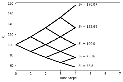
To get these values in Python we can use the following to get the terminal stock prices and option values at each node.
N = 4
S0  = 100
T = 0.5
sigma = 0.4
dt = T/N
K =105
r = 0.05
u = np.exp( sigma * np.sqrt(dt) )
d =  np.exp( -sigma * np.sqrt(dt) )
p = ( np.exp(r*dt) - d) / (u -d)

for k in reversed(range(N+1)):
    ST = S0 * u**k * d ** (N-k)
    print(round(ST,2), round(max(ST-K,0),2))


#176.07 71.07
#132.69 27.69
#100.0 0
#75.36 0
#56.8 0
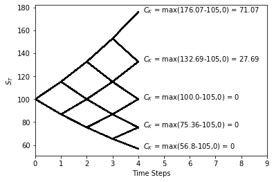
The probability at each node \(p^*\) is given by the following. Let k be the number of up moves in the stock.
\(p^* = \binom{N}{k}\ p^k (1-p)^{N-k} = \binom{N}{k}\ (\frac{e^{(r\Delta t) - d}}{u -d})^k (1- \frac{e^{(r\Delta t) - d}}{u -d} )^{N-k}\)
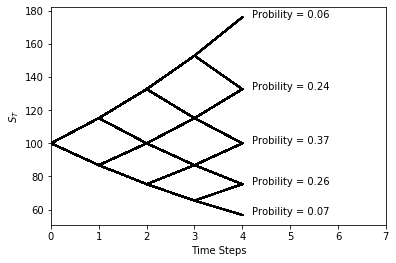
def combos(n, i):
    return math.factorial(n) / (math.factorial(n-i)*math.factorial(i))

for k in reversed(range(N+1)):
    p_star = combos(N, k)*p**k *(1-p)**(N-k)
    print(round(p_star,2))

#0.06
#0.24
#0.37
#0.26
#0.07
Finding the value of the call
The value of the call is then simply a weighted average of the values at each node multiplied by the corresponding probability value.
\(C_K = \displaystyle \sum_k^N \binom{N}{k}\ p^k (1-p)^{N-k}\ max(S_0\ u^k (d)^{N-k}-K,0)\)
C=0
for k in reversed(range(N+1)):
    p_star = combos(N, k)*p**k *(1-p)**(N-k)
    ST = S0 * u**k * d ** (N-k)
    C += max(ST-K,0)*p_star

print(np.exp(-r*T)*C)

#10.60594883990603
The full script from this section can be found at the end of the document labeled 'Rough work'
Let's put the script above into a function so that we can price puts also and also increase the step size \(\Delta t\) easily to see it's effect on the option price.
N =4
S0  = 100
T = 0.5
sigma = 0.4
K = 105
r = 0.05

def binom_EU1(S0, K , T, r, sigma, N, type_ = 'call'):
    dt = T/N
    u = np.exp(sigma * np.sqrt(dt))
    d = np.exp(-sigma * np.sqrt(dt))
    p = (  np.exp(r*dt) - d )  /  (  u - d )
    value = 0
    for i in range(N+1):
        node_prob = combos(N, i)*p**i*(1-p)**(N-i)
        ST = S0*(u)**i*(d)**(N-i)
        if type_ == 'call':
            value += max(ST-K,0) * node_prob
        elif type_ == 'put':
            value += max(K-ST, 0)*node_prob
        else:
            raise ValueError("type_ must be 'call' or 'put'" )

    return value*np.exp(-r*T)


binom_EU1(S0, K, T, r,sigma, N)

#10.605948839906029
The function above agrees with the price we got from the rough work section. We can now increase the number of steps to see the effect on the price of the call.
Notice that as we increase N the value of the call appears to converge towards $10.22. This price is actually the result we would get from the closed form Black Scholes formula.
Ns = [2, 4, 6, 8, 10, 20, 50, 100, 200, 300, 400,500, 600]


for n in Ns:
    c = binom_EU1(S0, K, T, r,sigma, n)
    print(f'Price is {n} steps is {round(c,2)}')


#Price is 2 steps is 9.99
#Price is 4 steps is 10.29
#Price is 6 steps is 10.35
#Price is 8 steps is 10.37
#Price is 10 steps is 10.37
#Price is 20 steps is 10.34
#Price is 50 steps is 10.27
#Price is 100 steps is 10.22
#Price is 200 steps is 10.22
#Price is 300 steps is 10.23
#Price is 400 steps is 10.22
#Price is 500 steps is 10.22
#Price is 600 steps is 10.22
Coin Flipping Option Model.
When we talk about a coin flipping option model, consider a stock that has a path determined by a coin that flips continuously between the date now and the expiration date, when the coin flips heads the stock goes up and when tails the stock goes down.
In fact what we are talking about here is taking the limit of the binomial model as we let \(\Delta t \rightarrow 0\) .
Consider what happens to the parameters of the model when this happens. Well, we will realize that \(u\) approaches 1 from the right, \(d \) approaches 1 from the left and the probability of an up move \( \frac{e^0-d}{u-d} \rightarrow 0.5\ \) so therefore this can be represented as a coin flip.
Let's consider taking one path of 100,000 flips keep the parameters of our model the same. Again we are not really taking the limit properly here, just a closer approximation, consider slicing the increments on the x axis into infinitely small increments to get an idea of the real limit.
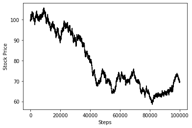
N=100000
sigma = 0.4
T = 0.5
K = 105
r= 0.05
dt = T / N
Heads = np.exp(sigma * np.sqrt(dt))
Tails = np.exp(-sigma * np.sqrt(dt))
S0 = 100
p = (  np.exp(r*dt) - Tails )  /  ( Heads - Tails )
paths = np.random.choice([Heads,Tails],p=[p,1-p],size=(N,1))
plt.plot(paths.cumprod(axis=0)*100, color='black');
plt.xlabel('Steps')
plt.ylabel('Stock Price')
So what has that got to do with the binomial model? Well perhaps when we create say 1000 such paths it will become clear. Note that this make take a while on your computer!!!!
paths = np.random.choice([Heads,Tails],p=[p,1-p],size=(N,1000))
plt.plot(paths.cumprod(axis=0)*100, color='black');
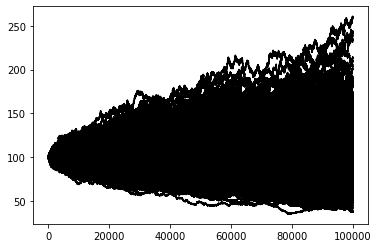
Consider being at step 100,000 above and taking the terminal values of the plot above. The payoff for a call would then become:
\(Call = \displaystyle \int_{K}^{\infty} payoff \ (S,K) dS\)
Now compare this to a lattice of suitable resolution as shown below. Notice that the lattice serves as an approximation to the continuous version above.
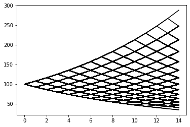
The continuous version is known as geometric Brownian motion, and in fact this is precisely what Cox, Ross and Rubinstein were approximating in their paper. Clearly the lattice method provides an accurate approximation of the price if the number of steps is large enough.
Pricing Real Options on Yahoo Finance.
In this section will will try out our model on data from Yahoo Finance, we showed previously how to interact with the options API. The issue we will likely have, is that we are pricing these options for TSLA using a European options expiry and the options themselves are highly likely to be American. We are also assuming a constant volatility of 50% (chosen for convenience.
Note that this data was taken on 21st December 2020. Obviously this will change if you the reader run the script again.
import pandas as pd
import pandas_datareader.data as web
import numpy as np
import datetime as dt
import math

import matplotlib.pyplot as plt


def combos(n, i):
    return math.factorial(n) / (math.factorial(n-i)*math.factorial(i))


def binom_EU1(S0, K , T, r, sigma, N, type_ = 'call'):
    dt = T/N
    u = np.exp(sigma * np.sqrt(dt))
    d = np.exp(-sigma * np.sqrt(dt))
    p = (  np.exp(r*dt) - d )  /  (  u - d )
    value = 0
    for i in range(N+1):
        node_prob = combos(N, i)*p**i*(1-p)**(N-i)
        ST = S0*(u)**i*(d)**(N-i)
        if type_ == 'call':
            value += max(ST-K,0) * node_prob
        elif type_ == 'put':
            value += max(K-ST, 0)*node_prob
        else:
            raise ValueError("type_ must be 'call' or 'put'" )

    return value*np.exp(-r*T)


def get_data(symbol):
    obj = web.YahooOptions(f'{symbol}')

    df = obj.get_all_data()

    df.reset_index(inplace=True)

    df['mid_price'] = (df.Ask+df.Bid) / 2
    df['Time'] = (df.Expiry - dt.datetime.now()).dt.days / 255

    return df[(df.Bid>0) & (df.Ask >0)]


df = get_data('TSLA')

prices = []


for row in df.itertuples():
    price = binom_EU1(row.Underlying_Price, row.Strike, row.Time, 0.01, 0.5, 20, row.Type)
    prices.append(price)


df['Price'] = prices

df['error'] = df.mid_price - df.Price


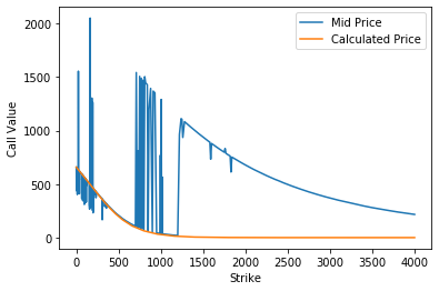
exp1 = df[(df.Expiry == df.Expiry.unique()[2]) & (df.Type=='call')]


plt.plot(exp1.Strike, exp1.mid_price,label= 'Mid Price')
plt.plot(exp1.Strike, exp1.Price, label = 'Calculated Price')
plt.xlabel('Strike')
plt.ylabel('Call Value')
plt.legend()
It seems that we haven't been able to replicate the options chain for this expiry very well. In the next few articles we will try to improve on this result. We will leave it to the reader to test on puts and at different expirations.
Rough Work
############params################
N = 4
S0  = 100
T = 0.5
sigma = 0.4
dt = T/N
K =105
r = 0.05
u = np.exp( sigma * np.sqrt(dt) )
d =  np.exp( -sigma * np.sqrt(dt) )
p = ( np.exp(r*dt) - d) / (u -d)


######showing terminal stock prices for 4 step model################

for k in reversed(range(N+1)):
    ST = S0 * u**k * d ** (N-k)
    print(round(ST,2), round(max(ST-K,0),2))


#176.07 71.07
#132.69 27.69
#100.0 0
#75.36 0
#56.8 0


############showing node probabilities
def combos(n, i):
    return math.factorial(n) / (math.factorial(n-i)*math.factorial(i))

for k in reversed(range(N+1)):
    p_star = combos(N, k)*p**k *(1-p)**(N-k)
    print(round(p_star,2))

#0.06
#0.24
#0.37
#0.26
#0.07


######valuing the call from example#######################

C=0
for k in reversed(range(N+1)):
    p_star = combos(N, k)*p**k *(1-p)**(N-k)
    ST = S0 * u**k * d ** (N-k)
    C += max(ST-K,0)*p_star

print(np.exp(-r*T)*C)

#10.60594883990603